In this article, we are going to define what VaR is, in relation to a portfolio of assets. We will go through the process of the calculation of the VaR for a particular example in step-by-step format. The Excel spreadsheet is presented bit by bit to allow for the explanation of each step and the commands related to each step.
What is VaR?
Suppose that we have an asset portfolio, that is, a group of assets. The value (or price) of each assets increases or decreases from one time (for example day or week or month) to the other. The VaR, which stands for Value-At-Risk, of a portfolio is the maximum amount that could be lost in a particular time horizon (for example in 1 day or in 5 days or in 3 months etc…) with a particular probability. For example, if the 5-day 95% VaR is equal to 100,000euro, this means that with a probability of 95%, the loss that could be suffered on the portfolio during a 5-day period will not be greater than 100,000euro. This associated probability value is also know as the level of confidence. The greater the time horizon the greater the VaR due to the increase in the uncertainty of the prices over a longer time period. Also the higher the level of confidence, the greater the VaR.
Worked Example
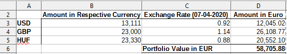
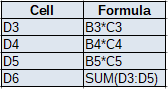
Suppose that we have three cash accounts in dollars, sterling and hungarian forint, with balances USD13111, GBP23000 and HUF23300 respectively. These are the three assets in our portfolio. Let our home currency be the euro. Thus the value of the portfolio (measured in euro) depends on the three exchange rates, namely USD to EUR, GBP to EUR, and HUF to EUR. These are the three prices of the three assets of the portfolio. Let’s say that we would like to know the largest loss that could be suffered in a 5-day period with a probability of 95%. In other words, we are after the 5-day 95% VaR of your portfolio.
Step 1: Calculating the current value of the portfolio
The balances in USD, GBP and HUF are converted to euro using the latest exchange rate (as at 7 April 2020 in our case).
Step 2: Calculating the weights
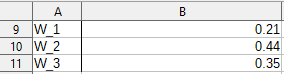
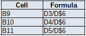
In Step 1, you have the balance of each asset in EUR and the total balance of the portfolio in EUR. Hence the proportion of the asset value (in EUR) over the total portfolio value (in EUR) is the weight of that asset. Note that the sum of weights is equal to 1.
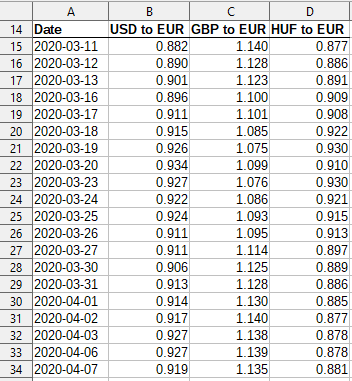
Step 3: Inputting a series of prices for each asset
In this example we have 20 daily prices for each asset available over the same time horizon. So at each time point we have the price for each asset. Not that in this example we are using daily prices. However you can also work with examples in which the prices are shown weekly, monthly etc… Just for demonstration of the method, we are working with just 20 prices. In reality you must either use all the data available that is relevant/adequate. Usually having one or two years of daily prices would be very good.
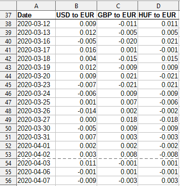
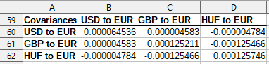
Step 4: Calculating the change in the prices
Here you can either choose to calculate the daily percentage changes or the daily logarithmic changes. A daily percentage change of an asset is its price of today minus its price of yesterday, all divided by its price of yesterday. A daily logarithmic change of an asset is the log value of the proportion of its price of today to its price of yesterday. In this example, we opt for the daily percentage changes.
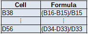
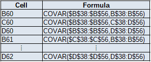
Step 5: Calculating the variance-covariance matrix
Here you calculate the variance-covariance matrix of the three series of percentage change. This captures the correlation structure between the changes in the prices of the three assets. The excel function used is the COVAR function but one could use the variance-covariance matrix option from the DataAnalysis Excel Add-In.
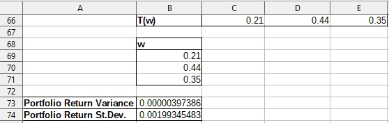
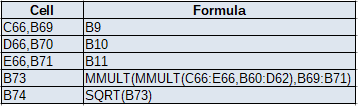
Step 6: Calculating the portfolio return variance and standard deviation
Mathematically, the portfolio return variance is given by the formula t(w) * A * w, where w is a column vector of the weights, t(w) is a row vector of the weights and A is the variance-covariance matrix. The portfolio return standard deviation is the square root of the portfolio return variance. The portfolio return standard deviation means that if you consider one portfolio return, you expect that it defers from the mean return (say mean return = 0%) by 0.2%.
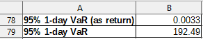
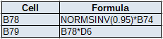
Step 7: Calculating the 1-day 95% VaR
The VaR presented in cell B78, is in return form. This is the z-value obtained from the normal distribution with a 95% confidence level multiplied by the portfolio return standard deviation. We expect a decrease of no more than 0.33% in one day with a confidence level of 95%. The VaR in cell B79 is presented in absolute terms. This means that we expect a decrease of no more than 192.49euro in one day with a level of confidence of 95%. In other example in which we require different level of confidence, say 90% or 99%, we put 0.9 or 0.99 inside the normsinv formula of cell B78.
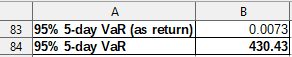
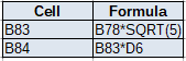
Step 8: Calculating the 5-day 95% VaR
The 5-day VaR is derived from 1-day VaR by applying the square root of time rule. Hence the multiplication by the square root of 5 in cell B83. Note that in other examples in which we are after other time horizons, say 2 weeks or 1 months, we multiply by the square root of 14 or the square root of 30 respectively.The resultant 95% 5-day VaR is 430.43euro.