Computing the Portfolio VaR using Copulas

In this article, we are going to model the combined distribution of the return prices of assets in a portfolio using copulas. This joint distribution will be then be used to work out the Value-At-Risk (VaR) of the portfolio. The advantages of this method, is that it relies on less assumptions than in the standard method of VaR computation, in which a multivariate normal distribution for the asset prices returns is assumed. In this method, we will choose a correlation structure (defined by a copula) that best fits the underlying data. The multivariate normal distribution will in fact be just one of these copulas that defines a particular correlation structure. Thus this improves the fit of the correlation structure and this added detail could avoid over-or-under estimation of the portfolio VaR. With the R software, we will work out the portfolio VaR using the copula that best fits the data and also compare it to the portfolio VaR figure given the usual multivariate normal distribution (or normal copula with normal marginals) is assumed.

Suppose that we have a portfolio of assets, which we shall call $X$ . Let $R$ denote the portfolio return in one time unit, that is, the percentage change in the total value of the portfolio in one time unit. Sometimes we would like to know the probability distribution of $R$ in order to get an idea of what values, the variable $R$ is likely to take. Or else, we would like to have an idea of how large the loss is expected to be given an unlikely bad scenario. This leads us to the definition of VaR. The $\alpha$ VaR of portfolio $X$ , is the greatest possible value of $r$ that satisfies:

$\begin{equation*} \mathbb{P}(R>r)\geq\alpha. \end{equation*}$

This means that with a probability of $\alpha$ , the return from the portfolio will be at least $r$ . For example, if the 95% VaR of the portfolio is -2%, this means that with a probability of 95%, the loss suffered will not be more than 2%.

In order to calculate the portfolio VaR, we must know the probability distribution of $R$ . However since a portfolio is made up of a number of assets and each of them have their own price, we will first show that $R$ is a weighted average of the returns of the individual assets. Suppose we have $n$ assets in the portfolio. Let $i \in \left\{ 1,2,\cdots,n \right\}$ . Let $X_i$ be the number of units of asset $i$ and $P_i$ be the price of each unit of asset $i$ . Let $V_i$ be the total value of asset $i$ . Hence $V_i=X_i P_i$ . Let $R_i$ be the rate of return from asset $i$ during one time unit (i.e. percentage change in the price of asset $i$ in one time unit) and let $S_i$ be the return from asset $i$ during one time unit (i.e. the profit or loss from asset $i$ during one time unit). Hence we have $S_i=V_iR_i$ .

The portfolio can be described by the set $X=\lbrace X_1,X_2,\cdots,X_n\rbrace$ . Let the total current value of the portfolio be $V$ , where $V=V_1+V_2+\cdots+V_n$ . The total return on the portfolio $S$ during one time unit is the sum of the return from each asset present in the portfolio. Thus $S=S_1+S_2+\cdots+S_n$ . Finally the rate of return $R$ on the whole portfolio is given by:

$\begin{equation*}\begin{split}R&=\frac{S}{V}\\ &=\frac{S_1+S_2+\cdots+S_n}{V}\\ &=\frac{V_1R_1+V_2R_2+\cdots+V_nR_n}{V}\\ &=\frac{V_1}{V} R_1+\frac{V_2}{V} R_2+\cdots+\frac{V_n}{V} R_n\\ &=w_1 R_1+w_2 R_2+\cdots+w_n R_n \end{split}\end{equation*}$

where $w_i=\frac{V_i}{V}$ for $i \in \left\{1,2,\cdots,n\right\}$ and represents the weight of asset $i$ in the portfolio at the current time.

Now the $\alpha$ VaR is the greatest possible value of $r$ satisfying:

$\begin{equation*} \mathbb{P}(w_1R_1+w_2R_2+\cdots+w_n R_n>r)\geq\alpha. \end{equation*}$

In order to work out the $\alpha$ VaR, we must know the joint distribution of $R_1,R_2,\cdots R_n$ . Note that each $R_i$ is univariate distribution and thus their joint distribution is an $n$ -variate distribution. Sklar’s Theorem proves that every multivariate distribution can expressed in terms of its marginal distribution and a copula. Thus the copula defines the correlation structure between the variables. For example, the multivariate normal distribution is constructed from marginal distributions that are all univariate normally distributed and a copula named “Gaussian”. However there are a number of other copulas, in particular, the Gumbel, the Frank, the Clayton and the Student t-Copulas. Each of them model the correlation structure between the variables in their unique way. For more details on how copulas model the correlation structure in the bivariate case, click here. Moreover, we are free to choose different distributions for the marginals. For example, we can construct a trivariate distribution from a Gaussian copula with the t-distribution, the gamma distribution and the normal distribution as the three marginals.

So here, we will fit a univariate distribution to each $R_i$ . Then we will choose a copula that best fits the data of the $R_i$ ‘s. Hence like this the multivariate distribution would be constructed and the VaR value could be found. Let us give an example of a portfolio with two stocks.

Let the two stocks be Facebook and PayPal which are available on the NASDAQ stock market, with the names “FB” and “PYPL” respectively. We consider their prices during a two-year time window from 1st January 2018 to the 31st December 2019. The prices can be inputted directly into the R software using the package “quantmod” and plotted.

library(quantmod)

start<-format(as.Date("2018-01-01"),"%Y-%m-%d")
end<-format(as.Date("2019-12-31"),"%Y-%m-%d")

Facebook<-getSymbols('FB', src= "yahoo", from=start, to=end, auto.assign = F)
PayPal<-getSymbols('PYPL', src= "yahoo", from=start, to=end, auto.assign = F)

par(mfrow=c(1,2))
ts.plot(FacebookPYPL.Adjusted,main="PYPL Stock Price",ylab="PYPL Stock Price")
par(mfrow=c(1,1))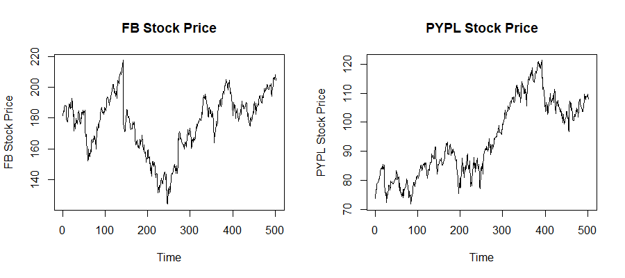

The percentage changes in the stock prices (the returns) are computed using the function “dailyReturn” and their histogram is plotted. The set of returns of Facebook is labelled “x” and the set of returns of PayPal is labelled “y”.

x<-as.vector(dailyReturn(Facebook))
y<-as.vector(dailyReturn(PayPal))

par(mfrow=c(1,2))
hist(x,main="Daily Returns of FB Histogram",xlab="FB Daily Returns")
hist(y,main="Daily Returns of PYPL Histogram",xlab="PYPL Daily Returns")
par(mfrow=c(1,1))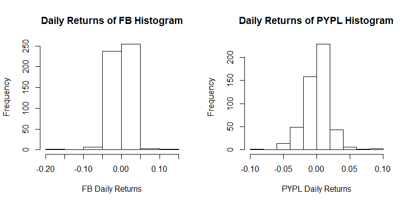

The shape of the histograms is more or less symmetric. So let us check whether a normal distribution is appropriate as the marginal distribution for any of these two stock returns. We use the Shapiro-Wilk test for normality. As a rule of thumb, a $p$ -value larger than 0.05 indicates that the normal distribution offers an appropriate fit for the data.

shapiro.test(x)
shapiro.test(y)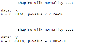

The distribution of the returns of both stocks deviates from normality. Hence we must find another distribution to fit our data. Let us consider some descriptive statistics of the returns, which are grouped in the table below, in order to understand more the underlying distribution.

#descriptives of FB Returns

library(e1071) #package for skewness and kurtosis functions

mean(x)
sd(x)
skewness(x)
kurtosis(x)

#descriptives of PYPL Returns

mean(y)
sd(y)
skewness(y)
kurtosis(y)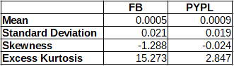

Both means are close to zero. Both stock returns display a high value of kurtosis, that is, they have fat tails. This is the most probably reason why the normal distribution is not accepted in the Shapiro-Wilk test. The skewness of the PayPal returns is close to zero. On the other hand we have a significant negative value for the skewness of the Facebook returns. However a closer look at the data indicates that this results from one very low return equal to -18.96%. In fact the removal of this outlier, results in a skewness of 0.179. Hence we can assume that the distribution of the Facebook returns is also symmetric. In the Cullen and Frey graph, the square of skewness and the kurtosis of the data is plot (as a blue dot) and compared to those of theoretical distributions.

library(fitdistrplus)

par(mfrow=c(1,2))
descdist(x, discrete=FALSE, boot=50)
descdist(y, discrete=FALSE, boot=50)
par(mfrow=c(1,1))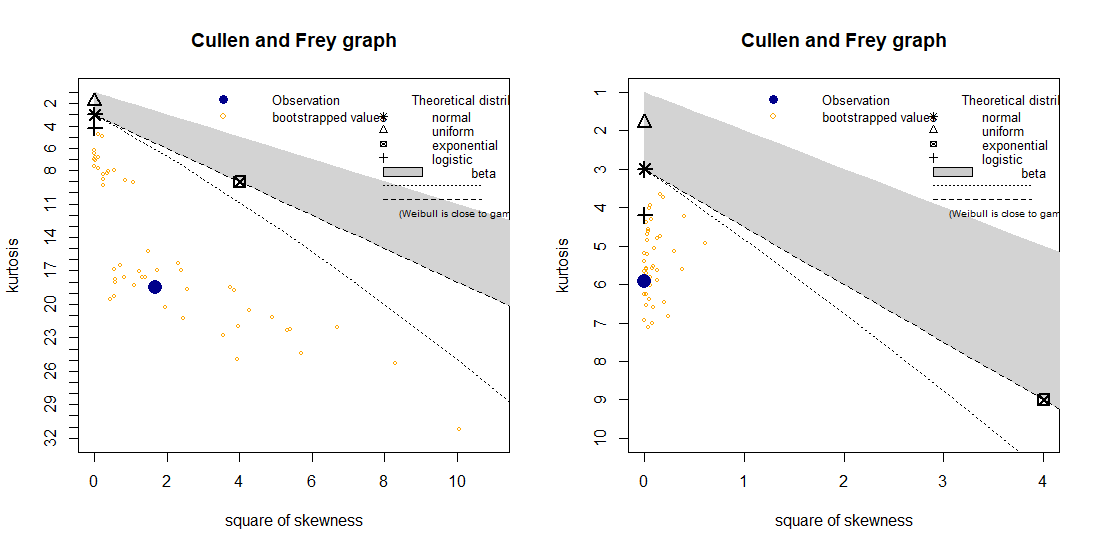

Since we are looking for distributions which have low or zero skewness, the closest one offered in the Cullen and Frey graph is the logistic distribution. However another distribution which we will consider is the $t$ -distribution which is used a lot in modelling stock returns. The package “QRM” is used to fit a $t$ -distribution to the stock returns. If $X$ is a random variable, the function “fit.st” outputs values for the parameters $\nu$ , $\mu$ , and $\sigma$ . The cumulative distribution function (c.d.f) of $X$ is $G(x)=F(\frac{x-\mu}{\sigma})$ where $F$ is the c.d.f. of the $t$ -distribution with $\nu$ d.o.f. By differentiating $G$ , it also follows that the fitted probability density function (p.d.f.) of $X$ is $g(x)=\frac{1}{\sigma}f(\frac{x-\mu}{\sigma})$ where $f$ is the p.d.f. of the $t$ -distribution with $\nu$ d.o.f. The inverse cumulative distribution of $X$ is $G^{-1}(x)=\sigma F^{-1}(x)+\mu$ .

The fitted t-distribution and the fitted normal distribution are drawn on the histograms in blue and red respectively.

#fitting the t distribution to FB Returns

library(QRM)

tfit1 <- fit.st(x)
#tfit1
tpars1<-tfit1[[2]] #vector of parameter estimates

nu1<-tpars1[1]
mu1<-tpars1[2]
sigma1<-tpars1[3]

par(mfrow=c(1,2))
z<-seq(-0.1,0.1,0.001)
hist(x,nclass=20,probability=TRUE,main = "Histogram of FB Returns",ylim=c(0,30),xlab="FB Returns")
a<-Vectorize(function(z) dnorm(z, mean=mean(x), sd=sd(x)))
curve(a, col="red", lwd=3,  add=TRUE)
b<-Vectorize(function (z) dt((z-mu1)/sigma1,df=nu1)/sigma1)
curve(b, col="blue", lwd=3,  add=TRUE)

#fitting the t distribution to PYPL Returns

tfit2 <- fit.st(y)
#tfit2
tpars2 <- tfit2[[2]] #vector of parameter estimates

nu2<-tpars2[1]
mu2<-tpars2[2]
sigma2<-tpars2[3]

z<-seq(-0.1,0.1,0.001)
hist(y,nclass=20,probability=TRUE,main = "Histogram of PYPL Returns",xlab="PYPL Returns")
a<-Vectorize(function(z) dnorm(z, mean=mean(y), sd=sd(y)))
curve(a, col="red", lwd=3,  add=TRUE)
b<-Vectorize(function (z) dt((z-mu2)/sigma2,df=nu2)/sigma2)
curve(b, col="blue", lwd=3,  add=TRUE)
par(mfrow=c(1,1))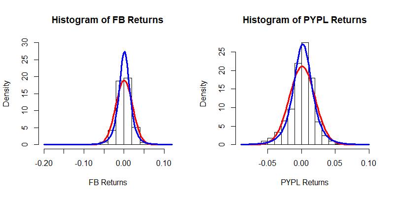

We can check the adequacy of each fit through the Kolmogorov-Smirnov test. First let us consider the distribution of the Facebook Returns. The first test checks whether the data follows a normal distribution and the second test checks whether the data follows a $t$ -distribution. Their results show that the $t$ -distribution provides a better fit for the data.

#Kolmogorov-Smirnov Test for FB

ks.test(x, "pnorm",mean=mean(x),sd=sd(x))

shiftedt<-function(k,nu,mu,sigma){pt((k-mu)/sigma,df=nu)}
ks.test(x, "shiftedt",nu=nu1,mu=mu1,sigma=sigma1)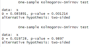

The same test is repeated for the PayPal data.

#Kolmogorov-Smirnov Test for PYPL
ks.test(y, "pnorm",mean=mean(x),sd=sd(x))

shiftedt<-function(k,nu,mu,sigma){pt((k-mu)/sigma,df=nu)}
ks.test(y, "shiftedt",nu=nu2,mu=mu2,sigma=sigma2)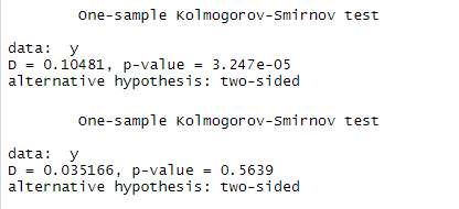

Now let us analyse the correlation structure between the two series of returns. On the left, we have a scatter plot of the Facebook returns and the PayPal Returns. Given that we will be fitting a distribution for each marginal, we can eliminate the marginals by considering the cumulative distribution functions of the returns series. We thus have the plot on the right, which still captures the correlation structure between the two variables. In this plot we see that there is some more point density in the bottom left than in the top right. This indicates that their might be stronger correlation between the negative tails than between the positive tails of the distributions.

par(mfrow=c(1,2))
plot(x,y,xlab="FB Daily Returns",ylab="PYPL Daily Returns",main="FB and PYPL Daily Returns Scatterplot")

xtrans<-ecdf(x)(x)
ytrans<-ecdf(y)(y)
plot(xtrans,ytrans,xlab="CDF FB Daily Returns",ylab="CDF PYPL Daily Returns",main="FB and PYPL Returns CDFs")
par(mfrow=c(1,1))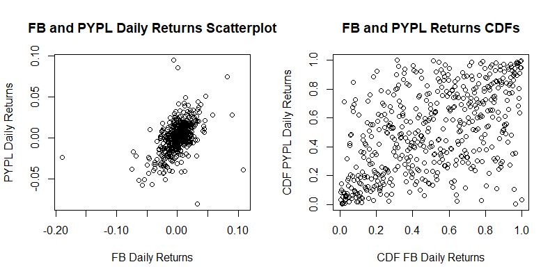

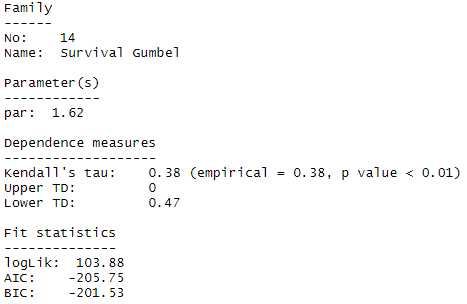
Next we use the function “BiCopSelect” from the package “VineCopula” which chooses a copula that best fits the data by considering the AIC and BIC criteria.

library(VineCopula)

FittedCopula<-BiCopSelect(xtrans,ytrans,familyset=NA)
summary(FittedCopula)

The chosen copula is called the “Survival Gumbel” copula which is also known as the rotated Gumbel copula. This is in fact one of the copulas that has higher dependency in the negative tails than in the positive tails.

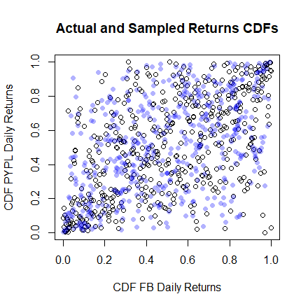
We can produce a random sample from this copula in order to get a rough idea whether the chosen copula is appropriate in this particular case. The random sample (displayed by the light blue dots) is generated with the formula “BiCopSim”, again from the package “VineCopula”.

plot(xtrans,ytrans,xlab="CDF FB Daily Returns",ylab="CDF PYPL Daily Returns",main="Actual and Sampled Returns CDFs")

CopulaSim<-BiCopSim(length(x), FittedCopulapar)
points(CopulaSim, col = rgb(0,0,1,alpha=0.3), pch=16)

In this plot we see that the actual data and the sample data seem to have similar distribution, because they both cover the $[0,1]^2$ area in a similar fashion.

So till now we have modeled the two marginal distributions and the correlation structure via a copula. Thus, by Sklar’s Theorem, we can say that we have the bivariate distribution of these two stock returns defined. Hence we are now ready to compute the VaR of the portfolio. Let us assume that the current value of portfolio is made up of 70% Facebook stocks and 30% PayPal stocks. We compute the 99% Portfolio VaR as follows. We generate a large sample (of size 1,000,000) of possible values of $R_1$ and $R_2$ (returns of Facebook and PayPal stocks), and compute the 1st percentile of $w_1R_1+w_2R_2$ . This is repeated 20 times and the average of the percentiles is taken to be the 99% VaR.

#Portfolio Weights
w1<-0.7 
w2<-0.3

library(copula)
library(VC2copula)

n<-1000000
Percentiles<-c()
for(i in 1:20)
{sim<-rCopula(n,copulaFromFamilyIndex(FittedCopulapar))
sim2<-cbind(qt(sim[,1],df=nu1)*sigma1+mu1,qt(sim[,2],df=nu2)*sigma2+mu2)
Percentiles<-c(Percentiles,sort(sim2 %*% c(w1,w2))[0.01*n])}

VaR<-mean(Percentiles)
VaR

We obtain a 1-day 99% VaR of -4.94% for this portfolio. Let us make a comparison with the VaR figure obtained when the underlying distribution is assumed to be the multivariate normal distribution, that is, having normally distributed marginals with the Gaussian (or normal) copula.

#Computing VaR with the Multivariate Normal Distribution
n<-1000000
Percentiles<-c()
for(i in 1:20)
{sim<-rCopula(n,normalCopula(param = cor(x,y), dim = 2))
sim2<-cbind(qnorm(sim[,1],mean=mean(x),sd=sd(x)),qnorm(sim[,2],mean=mean(y),sd=sd(y)))
Percentiles<-c(Percentiles,sort(sim2 %*% c(w1,w2))[0.01*n])}

VaR<-mean(Percentiles)
VaR

In this case we obtain a 1-day 99% VaR of -4.18%, an increase of 0.76% from the previous calculation.

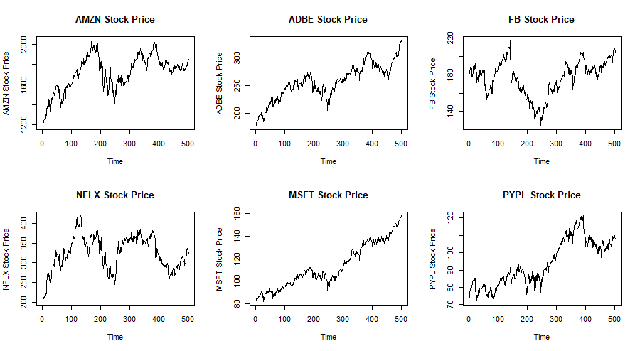
This method could be extended to work on a portfolio with more than just two stocks. Since the number of calculations and lines of code will naturally increase, the relevant R code will be shown at the end as an appendix. Suppose we have a portfolio made up of 6 stocks namely Amazon, Adobe, Facebook, Netflix, Microsoft and PayPal. These are all traded on NASDAQ by the acronyms AMZN, ADBE, FB, NFLX, MSFT and PYPL respectively. The following are the plots of the prices of these stocks during the two-year period from 1 January 2018 to 31 December 2019.

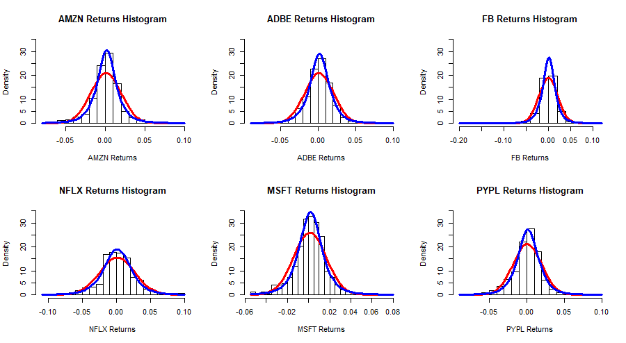
The daily returns of the 6 stocks is computed and shown in histograms with two superimposed curves. The red curve is a fitted normal distribution and the blue curve is a fitted t-distribution. The plots together with the Kolmorogov-Smirnov tests show that the $t$ -distribution offers a better fit for the marginals.

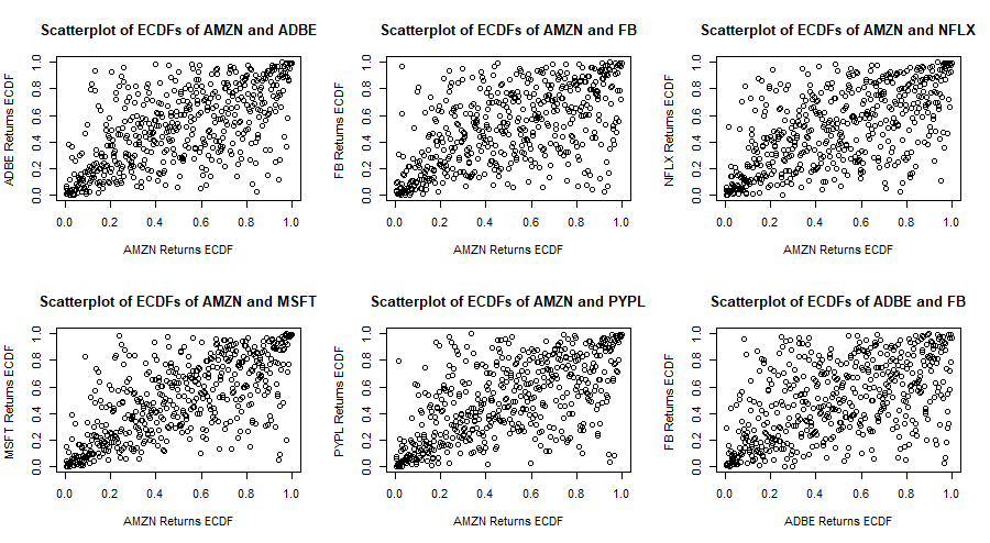
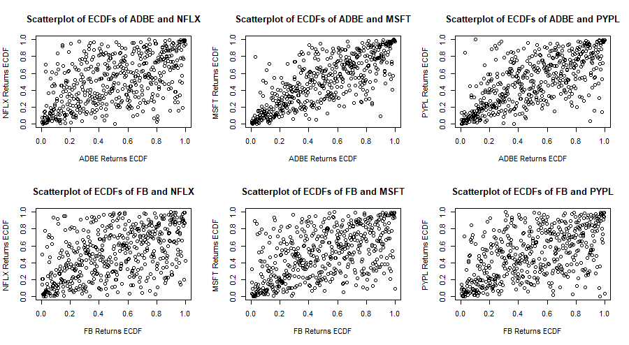
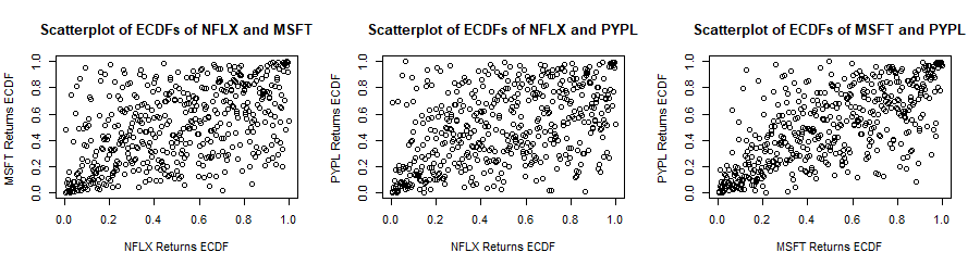
Now that a $t$ -distribution is fitted to each marginal distribution, each series of returns is transformed to a series of empirical c.d.f. values. The following are scatterplots of empirical c.d.f. values of pairs of stock returns. In general there is some stronger correlation in the tails of the distributions and the correlation in the negative tails seems stronger than that in the positive tails. In fact the bivariate copula that fits best each of these pairs of e.c.d.f.s (according to the AIC and BIC criteria) is the survival (or rotated) Gumbel copula.

We now “rotate” (transform) the data by considering new c.d.f.’s $F'$ where $F'=1-F$ . Thus the negative tails now become the positive tails and vice-versa. We fit a 6-dimensional Gumbel copula to these new c.d.f.’s.

Suppose for this example that the portfolio value is made up of 15% Amazon stocks, 15% Adobe stocks, 15% Facebook stocks, 15% Netflix stocks, 15% Microsoft stocks and 25% PayPal stocks. Hence the portfolio weights are $w_1=w_2=w_3=w_4=w_5=0.15$ and $w_6=0.25$ . The 99% 1-day portfolio VaR using the survival Gumbel copula and $t$ -distributed marginals is equal to -4.84%. As a comparison if we use the multivariate normal distribution, the 99% 1-day portfolio VaR is equal to -3.67%.

Conclusion

In this article, we have shown how to model the joint distribution of the asset returns of the portfolio through individually modelling the marginal distributions and the correlation structure via a copula. Various plots and the Kolmogorov-Smirnov Test are used to assess the appropriateness of the fitted marginal distributions. The copula which provides the best fit is chosen on basis of the AIC and BIC criteria. Once the joint distribution is modelled, the 99% Portfolio VaR is found. Moreover this result is compared to the 99% Portfolio VaR given the multivariate normal distribution is used.

Appendix

In this appendix we show the R code used to compute the VaR of a portfolio of 6 stocks together with some explanations. The code below is used to import the stock prices into R and plot these series.

library(quantmod)

start<-format(as.Date("2018-01-01"),"%Y-%m-%d")
end<-format(as.Date("2019-12-31"),"%Y-%m-%d")

Amazon<-getSymbols('AMZN', src= "yahoo", from=start, to=end, auto.assign = F)
Adobe<-getSymbols('ADBE', src= "yahoo", from=start, to=end, auto.assign = F)
Facebook<-getSymbols('FB', src= "yahoo", from=start, to=end, auto.assign = F)
Netflix<-getSymbols('NFLX', src= "yahoo", from=start, to=end, auto.assign = F)
Microsoft<-getSymbols('MSFT', src= "yahoo", from=start, to=end, auto.assign = F)
PayPal<-getSymbols('PYPL', src= "yahoo", from=start, to=end, auto.assign = F)

par(mfrow=c(2,3))
ts.plot(AmazonADBE.Adjusted,main="ADBE Stock Price",ylab="ADBE Stock Price")
ts.plot(FacebookNFLX.Adjusted,main="NFLX Stock Price",ylab="NFLX Stock Price")
ts.plot(MicrosoftPYPL.Adjusted,main="PYPL Stock Price",ylab="PYPL Stock Price")
par(mfrow=c(1,1))

The following R code computes, the daily returns of the stocks and plots their histogram. The Shapiro-Wilk test is performed on all asset returns and confirms that they do not follow the normal distribution.

a<-as.vector(dailyReturn(Amazon))
b<-as.vector(dailyReturn(Adobe))
c<-as.vector(dailyReturn(Facebook))
d<-as.vector(dailyReturn(Netflix))
e<-as.vector(dailyReturn(Microsoft))
f<-as.vector(dailyReturn(PayPal))


par(mfrow=c(2,3))
hist(a,main="Daily Returns of AMZN Histogram",xlab="AMZN Daily Returns")
hist(b,main="Daily Returns of ADBE Histogram",xlab="ADBE Daily Returns")
hist(c,main="Daily Returns of FB Histogram",xlab="FB Daily Returns")
hist(d,main="Daily Returns of NFLX Histogram",xlab="NFLX Daily Returns")
hist(e,main="Daily Returns of MSFT Histogram",xlab="MSFT Daily Returns")
hist(f,main="Daily Returns of PYPL Histogram",xlab="PYPL Daily Returns")
par(mfrow=c(1,1))

shapiro.test(a)
shapiro.test(b)
shapiro.test(c)
shapiro.test(d)
shapiro.test(e)
shapiro.test(f)

The following R code fits a $t$ -distribution and also a normal distribution to each series of returns. The histogram of each series of returns is again plotted, the superimposed blue curve shows the fitted $t$ -distribution and the superimposed red line shows the fitted normal distribution. The Kolmogorov-Smirnov test is performed and shows that each series can be better described as following the $t$ -distribution.

library(QRM)

nu<-c()
mu<-c()
sigma<-c()
names<-c("AMZN","ADBE","FB","NFLX","MSFT","PYPL")
par(mfrow=c(2,3))

for(i in 1:ncol(data))
{
tfit <- fit.st(data[,i])
tpars <- tfit[[2]]

nu[i]<-tpars[1]
mu[i]<-tpars[2]
sigma[i]<-tpars[3]

z<-seq(-0.1,0.1,0.001)
hist(data[,i],nclass=20,probability=TRUE,ylim=c(0,35),main=paste(as.character(names[i]),"Returns Histogram"),xlab=paste(as.character(names[i]),"Returns"))
a<-Vectorize(function(z) dnorm(z, mean=mean(data[,i]), sd=sd(data[,i])))
curve(a, col="red", lwd=3,  add=TRUE)
b<-Vectorize(function (z) dt((z-mu[i])/sigma[i],df=nu[i])/sigma[i])
curve(b, col="blue", lwd=3,  add=TRUE)

print(ks.test(data[,i], "pnorm",mean=mean(data[,i]),sd=sd(data[,i])))

shiftedt<-function(k,nu,mu,sigma){pt((k-mu)/sigma,df=nu)}
print(ks.test(data[,i], "shiftedt",nu=nu[i],mu=mu[i],sigma=sigma[i]))
}
par(mfrow=c(1,1))

The data frame “data” which contains the series of returns is transformed to the dataframe “datatrans” which contains the empirical c.d.f.s of each series. The scatterplots of pairs of emprical c.d.f.s of series are plotted.

datatrans<-data
for(i in 1:ncol(data)){datatrans[,i]<-ecdf(data[,i])(data[,i])}

par(mfrow=c(2,3))
for(i in 1:(ncol(datatrans)-1))
{for(j in (i+1):ncol(datatrans))
{plot(datatrans[,i],datatrans[,j],xlab=paste(as.character(names[i]),"Returns ECDF"),ylab=paste(as.character(names[j]),"Returns ECDF"),main=paste("Scatterplot of ECDFs of",as.character(names[i]),"and",as.character(names[j])))}}
par(mfrow=c(1,1))

The following fits the most appropriate bivariate copula to each pair of empirical c.d.f.s values of the returns.

library(VineCopula)

for(i in 1:(ncol(datatrans)-1))
{for(j in (i+1):ncol(datatrans))
{summary(BiCopSelect(datatrans[,i],datatrans[,j],familyset=NA))}}

The data is transformed or “rotated” in order for the positive tails to the become the negative tails and vice-versa, and a 6D copula is fitted to this data.

library(copula)

rotateddata<-1-datatrans
fit<-fitCopula(gumbelCopula(dim=6), as.matrix(rotateddata), method="itau")
fit

The vector $w$ is the vector of weights of the assets in the portfolio. The following code computes the 99% 1-day VaR first by using a 6D survival Gumbel copula and t-distributed marginal, and then by using a 6D normal distribution.

w<-c(0.15,0.15,0.15,0.15,0.15,0.25)

#Survival Gumbel and t-distributed marginals

n<-1000000
Percentiles<-c()
for(i in 1:20)
{
sim<-rCopula(n,gumbelCopula(1.791,dim=6))
sim<-1-sim

sim2<-as.matrix(qt(sim[,1],df=nu[1])*sigma[1]+mu[1])
for(i in 2:6)
{sim2<-cbind(sim2,qt(sim[,i],df=nu[i])*sigma[i]+mu[i])}
Percentiles<-c(Percentiles,sort(sim2 %*% w)[0.01*n])
}

VaR<-mean(Percentiles)
VaR

#Multivariate normal distribution

library(mvtnorm)

n<-1000000
Percentiles<-c()
for(i in 1:20)
{sim<-rmvnorm(n, mean=colMeans(data), sigma=var(data), method="chol")
Percentiles<-c(Percentiles,sort(sim %*% w)[0.01*n])}

VaR<-mean(Percentiles)
VaR