Common Questions about the Normal Distribution

Common Questions about the NOrmal Distribution

Introduction

In this article, various questions regarding the normal distribution are answered. The effects of the mean and the standard deviation on the shape of the normal distribution are analysed. We will describe how to obtain probabilities of intervals and on the other hand how to construct confidence intervals for a certain level of confidence. The 1-tailed and 2-tailed $z$ -scores are defined and we show how any normal distribution could be transformed into a standard normal distribution.

What determines the shape of the normal distribution?

The shape of the normal distribution resembles that of a bell. It is perfectly symmetric and is described completely by two parameters: $\mu$ the mean and $\sigma^2$ the variance. Equivalently, instead of the variance $\sigma^2$ , one could use the standard deviation $\sigma$ as the parameter that describes the normal distribution. The standard deviation is simply the positive square root of the variance. Note that $\sigma$ is always taken to be a positive number.

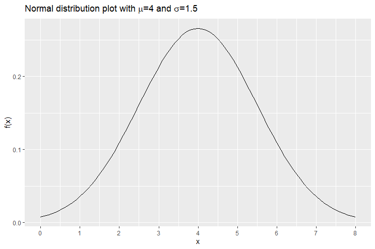
The graph of the normal distribution reaches its peak at $x=\mu$ . The graph decreases to 0 as $x\rightarrow\infty$ . However it never reaches 0. In other words, the graph never touches the $x$ -axis. On the other hand, the graph decreases to 0 as $x\rightarrow -\infty$ . Again it never reaches 0. In other words, the $x$ -axis is said to be an asymptote to the graph. The following is a plot of the normal distribution with $\mu=4$ and $\sigma=1.5$ . The graph reaches the peak at $x=\mu=4$ .

The following is the plot of the normal distribution with mean $\mu=0$ and standard deviation $\sigma=1$ . The normal distribution with these exact two values ( $\mu=0$ and $\sigma=1$ ) is known specifically by the name: standard normal distribution. The standard normal distribution reaches its peak when $x=0$ and is symmetric about the $x$ -axis.

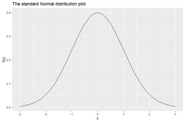
It is important to note that the curve of the normal distribution never cuts off. It continues indefinitely as $x\rightarrow\infty$ and $x\rightarrow -\infty$ . Another intrinsic property of the normal distribution is that the area of under the curves is always equal to 1, no matter the choice of $\mu$ and $\sigma$ .

What is the effect of the mean $\mu$ on the shape of the normal distribution?

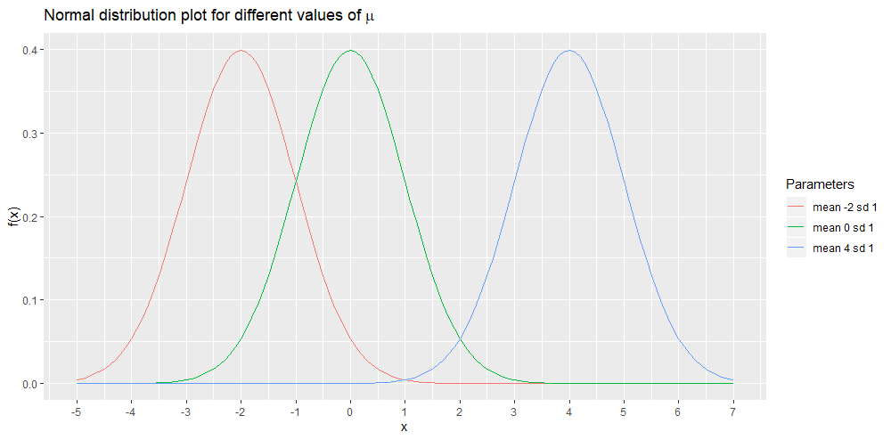
As we already mentioned, the graph of the normal distribution reaches its peak at $x=\mu$ . Hence when we change the value of $\mu$ , we are changing the location where the graph reaches its peak. In other words, we are shifting the graph horizontally (along the $x$ -axis). The shape per se, is left intact with a change in the value of $\mu$ . The following is a plot of three different normal distributions. They all have their standard deviation equal to 1. However they have different values for the means. The red curve has mean -2, the green curve has mean 0 and the blue curve has mean 4.

What is the effect of the standard deviation $\sigma$ on the shape of the normal distribution?

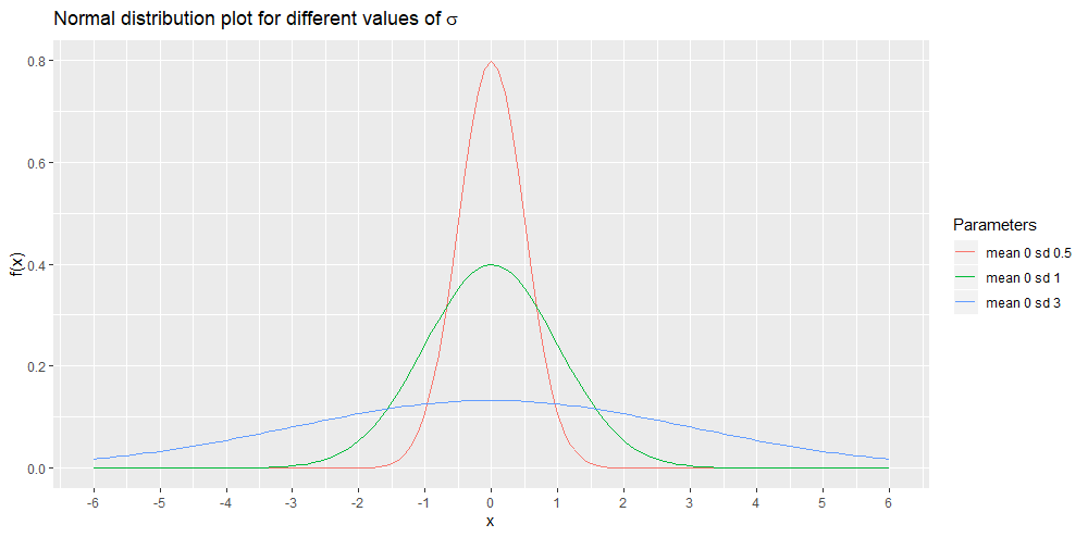
In contrast to the mean, the standard deviation actually changes the shape of the distribution although the shape would always remain bell-like and symmetric. The next plot shows three normal distributions. They all have mean 0 but different values of $\sigma$ . A small value of $\sigma$ results is a graph that has a higher peak but more narrow tails (left-most and right-most parts of the curve). This fact is demonstrated by the red curve. A smaller value of $\sigma$ results is a graph that has a higher peak but more narrow tails (left-most and right-most parts of the curve). This fact is shown by the red curve. A higher value of $\sigma$ results is a graph that has a lower peak but wider tails. This is demonstrated by the blue curve.

What does it mean that a random variable is normally distributed?

Suppose you have a random variable. This is a variable that takes on a particular real number in a random fashion according to some probability distribution. A well- known probability distribution is the uniform distribution. If, for example, a random variable follows a uniform distribution on the interval [0,1], it means that $X$ can take on a value between 0 and 1, and each number between 0 and 1, has the same probability (chance) of being selected (hence the name uniform distribution).

Now, a normally-distributed random variable $X$ is a random variable $X$ which takes on values depending on the normal distribution. Since $X$ is a real number and thus can theoretically take any number from $-\infty$ to $\infty$ , the probability is defined on intervals rather than points. The probability that $X$ takes a value between $a$ and $b$ is equal to the area under the curve between $x=a$ and $x=b$ .

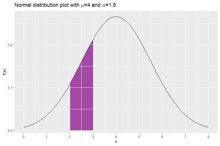
Consider for example a random number $X$ that follows the normal distribution with $\mu=4$ and $\sigma=1.5$ . Suppose that we would like to find the probability that $X$ takes on a value between 2 and 3.

Let us plot again the graph of the normal distribution with mean 4 and standard deviation 1.5. We would like to find the area enclosed by the normal distribution, the $x$ -axis and the vertical lines $x=2$ and $x=3$ . This is the area shaded in purple below and gives us the probability that $X$ lies between 2 and 3. The area is 0.161, hence we write $\mathbb{P}[2\leq X \leq 3]= 16.1\%$

Why is the mean $\mu$ called a measure of location?

The mean $\mu$ gives an idea of where the realisation of $X$ is expected to be. If, for example, we have a normally-distributed random variable with mean $4$ , we expect that it will take some value around 4 for most of the time.

Due to the symmetric bell-shape of the distribution, the mean of the normal distribution is equal to the median (since it is symmetric) and the mode (since it reaches the peak at $\mu$ ).

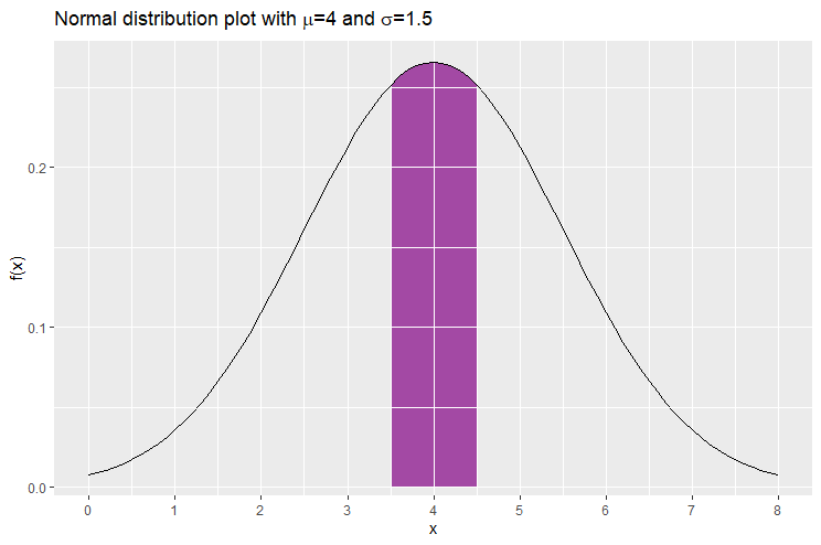
Moreover if you consider all the interval of same length, say $k$ , the interval which has the highest probability of containing the value of $X$ is $[\mu-\frac{k}{2},\mu+\frac{k}{2}]$ . For example if $X$ is again normally-distributed with mean 4 and standard deviation 1.5, and we let $k$ to be 1, the interval of length 1 carrying the largest probability is [3.5,4.5], where $\mathbb{P}[3.5\leq X \leq 4.5]= 26.1\%$ . This associated area is displayed in purple below.

Which are the most common $z$ -scores?

A random variable that follows the standard normal distribution is commonly denoted by the letter $Z$ instead of $X$ . This is just an issue of notation. Hence let us consider the random variable $Z$ that follows the standard normal distribution.

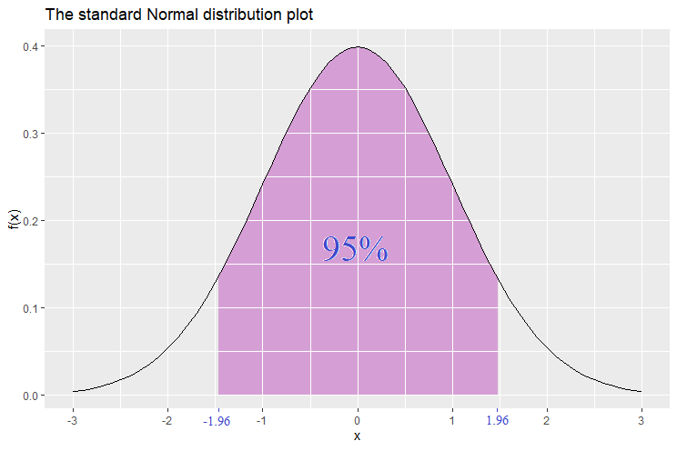
Suppose that we want to find an interval around the mean 0 (that is, $\mu=0$ is the center of the interval) that has a probability of 95%. The interval is found to be [-1.96,1.96]. Hence $\mathbb{P}[-1.96\leq Z\leq 1.96]=95\%$ . Hence we are 95% confident that $Z$ takes on a value between -1.96 and 1.96. The values -1.96 and 1.96 are called the 2-tailed 95% confidence level $z$ -scores. We call them 2-tailed because the shaded area in the graph below is concentrated in the middle part, and this leaves the two tails unshaded.

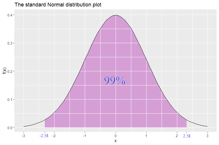
Similarly, let’s find the interval around the mean that carries a probability of 99%. This is found to be [-2.58,2.58]. Hence $\mathbb{P}[-2.58\leq Z\leq 2.58]=99\%$ . The values -2.58 and 2.58 are called the 2-tailed 99% confidence level $z$ -scores.

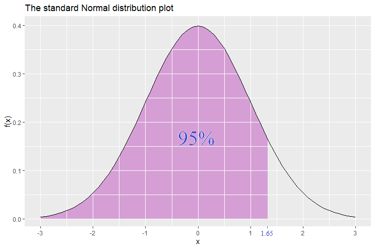
On the other hand there are also the 1-tailed $z$ -scores related to the 95% and 99% confidence level. Let’s start with the 95% confidence level. The shaded area starts from the left and only the right tail is unshaded. The area of the shaded part is 95%. The $z$ -value where the shaded part stops is 1.65. Hence we have found that the probability that $Z$ takes a value less than (or equal) to 1.65 is 95%, that is, $\mathbb{P}[Z\leq 1.65]=95%$ . The value 1.65 is called the 1-tailed 95% confidence level $z$ -score.

Similarly, the 1-tailed 99% confidence level $z$ -score is 2.33. Hence $\mathbb{P}[Z\leq 2.33]=99%$ .

Since the normal distribution is symmetric, it follows that $\mathbb{P}[Z\geq -2.33]=99\%$ and this could be demonstated by a plot in which the shaded part starts from the right side and leaves the left tail unshaded.

How are the $z$ -scores extended to be used for any normal distribution?

Consider the 2-tailed $z$ -scores. We have found that

$\begin{equation*} \mathbb{P}[-z\leq Z\leq z]=\alpha, \end{equation*}$

where $\alpha$ is the associated level of confidence (the probability of the interval). Every normal distributed random variable can be transformed into a standard normal distribution, through the equation:

$\begin{equation*} Z=\frac{X-\mu}{\sigma}. \end{equation*}$

Hence:

$\begin{equation*} \begin{split} \mathbb{P}[-z\leq Z\leq z]&=\alpha\\ \mathbb{P}[-z\leq \frac{X-\mu}{\sigma} \leq z]&=\alpha\\ \mathbb{P}[\mu-z\sigma\leq X \leq \mu+z\sigma]&=\alpha \end{split} \end{equation*}$

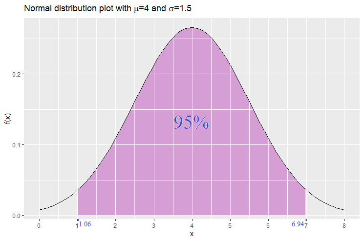
For example, let $X$ be normally distributed with mean 4 and standard deviation 1.5. Suppose that we would like to find the interval that carries a probability of 95%. We will thus make use of the 2-tail 95% $z$ -scores (-1.96 and 1.96).

$\begin{equation*} \begin{split} \mathbb{P}[\mu-z\sigma\leq X \leq \mu+z\sigma]&=\alpha\\ \mathbb{P}[4-1.96(1.5)\leq X \leq 4+1.96(1.5)]&=95\%\\ \mathbb{P}[1.06\leq X \leq 6.94]&=95\% \end{split} \end{equation*}$

Hence the interval we expect that $X$ takes on a value between 1.06 and 6.94 with probability 95%. The plot below displays this result.

What is the 68-95-99.7 rule?

Let $X$ be a normally-distributed random variable with mean $\mu$ and standard deviation $\sigma$ . If we had to find out the intervals which have probability roughly equal to 68%, 95% and 99.7% we obtain:

$\begin{equation*} \begin{split} \mathbb{P}[\mu-\sigma\leq X \leq\mu+\sigma]&\simeq 68\%\\ \mathbb{P}[\mu-2\sigma\leq X \leq \mu+2\sigma]&\simeq 95\%\\ \mathbb{P}[\mu-3\sigma\leq X \leq \mu+3\sigma]&\simeq 99.7\% \end{split} \end{equation*}$

Thus with probability 68%, the realisation of $X$ is within 1 standard deviation away from the mean. With probability 95%, the realisation of $X$ is within 2 standard deviations away from the mean, and so on.

Why is the standard deviation $\sigma$ called a measure of spread/dispersion?

The standard deviation $\sigma$ gives an idea of how much the random variable is expected to vary from the mean. If you take a sample of realisations of $X$ , their difference from the mean $mu$ is expected to be around $\sigma$ . The standard deviation measure how much the data of $X$ is close or far (dispersed) from its mean.

Take two normally distributed random variables $X_1$ and $X_2$ that both have mean $\mu$ , but $X_1$ has standard deviation $\sigma_1$ and $X_2$ has standard deviation $\sigma_2$ where $\sigma_1<\sigma_2$ . Then the interval around the mean $\mu$ having an associated probability $\alpha$ has a shorter length for the random variable $X_1$ .

For example let $X_1$ be normally distributed with mean 0 and standard deviation 0.5, and let $X_2$ be normally distributed with mean 0 and standard deviation 3. Let $\alpha=95\%$ . Then we obtain:

$\begin{equation*} \mathbb{P}(-0.98\leq X_1 \leq 0.98)=95\%\mbox{ and }\mathbb{P}(-5.88\leq X_2\leq 5.88)=95\% \end{equation*}$

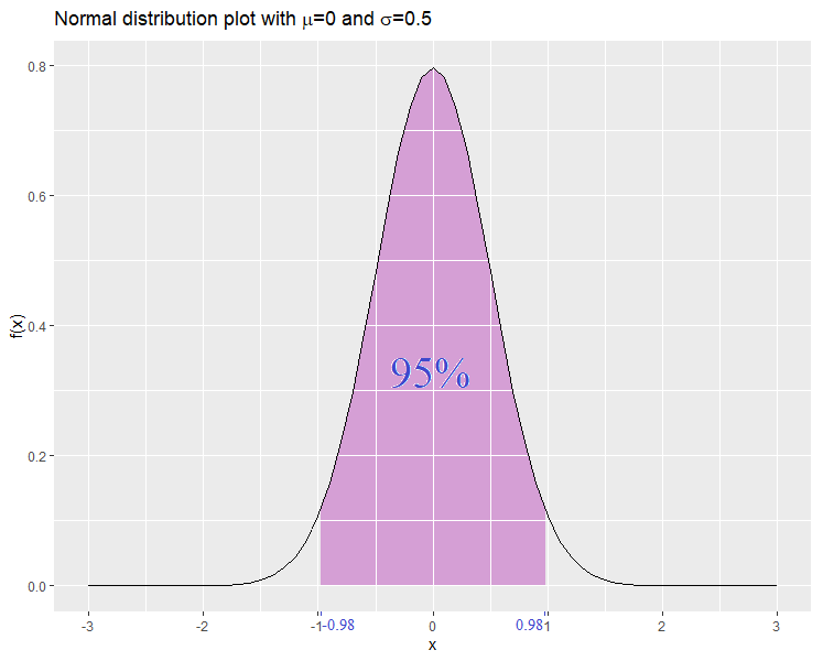
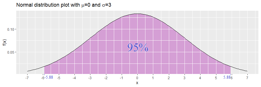
Since the interval for $X_1$ is shorter, then we have a clearer picture of which values are more likely to occur. This results from the fact that $X_1$ has a smaller standard deviation than $X_2$ .

What is the equation of the graph of the normal distribution?

The equation of the normal distribution is given by:

$\begin{equation*} f(x)=\frac{1}{\sqrt{2\pi\sigma^2}}e^{-\frac{(x-\mu)^2}{2\sigma^2}} \end{equation*}$

When entering various values for $\mu$ and $\sigma$ one would obtain different plots of the normal distribution as described above. The computations done to find the probabilities of interval, are carried out by finding the area under the graph through integration. Nowadays, statistical packages, like Excel and R, could work out these probabilities, and $x$ -values or $z$ -values very quickly through in-built functions.