3D & Contour Plots of the Bivariate Normal Distribution

3D and Contour Plots of

the Bivariate Normal Distribution

Introduction

In this article we are going to have a good look at the bivariate normal distribution and distributions derived from it, namely the marginal distributions and the conditional distributions. Sometimes the bivariate case is overlooked when the analysis shift directly from the univariate case to the multivariate case. However, the bivariate case helps us understand more the general multivariate case, especially with the use of 3D plots and contour plots. We will construct 3D graphs and contour plots with R, displaying the bivariate normal distribution for the cases where there is positive, negative and no correlation between the two variables. The effects of the means and the variances on the bivariate distribution are also analysed. In particular the case in which the two variables have equal variances is considered. The effect of correlation on the conditional distributions of the bivariate normal distribution is studied. This will lead to a study of copulas which offers a more general way how to combine two marginal distributions into one bivariate distribution. The R codes used to generate the plots in this article are provided in the appendix at the end.

The Univariate Normal Distribution

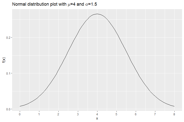
First let us consider the univariate normal distribution and then we will extend it to the bivariate normal distribution. Let $X$ be a normally distributed random variable with mean $\mu$ and standard deviation $\sigma$ (or variance $\sigma^2$ ). This is summarised by the notation $X\sim \mathcal{N}(\mu,\sigma^2)$ . The probability distribution of $X$ is given by:

$\begin{equation*} f(x)=\frac{1}{\sqrt{2\pi\sigma^2}}e^{-\frac{(x-\mu)^2}{2\sigma^2}} \end{equation*}$

This is called the univariate normal distribution because only one random variable ( $X$ ) is involved. The probability that $X$ takes on a value between $a$ and $b$ is given by:

$\begin{equation*} \mathbb{P}[a\leq X \leq b]= \int_{a}^{b} f(x)dx = \int_{a}^{b} \frac{1}{\sqrt{2\pi\sigma^2}}e^{-\frac{(x-\mu)^2}{2\sigma^2}}dx \end{equation*}$

If we let $\mu=4$ and $\sigma=1.5$ , $X$ has the probability distribution:

$\begin{equation*} f(x)=\frac{1}{\sqrt{2\pi(1.5^2)}}e^{-\frac{(x-4)^2}{2(1.5^2)}} \end{equation*}$

and if we plot this equation, we obtain:

You can have a look at an article dedicated solely to the univariate normal distribution, available here.

The Bivariate Normal Distribution

Let $X_1$ and $X_2$ be two normal random variable that have their joint probability distribution equal to the bivariate normal distribution. Let $X_1$ have mean $\mu_1$ and variance $\sigma_{11}$ . Let $X_2$ have mean $\mu_2$ and variance $\sigma_{22}$ . Let the covariance between $X_1$ and $X_2$ be $\sigma_{12}$ then their joint (bivariate) normal distribution is given by:

(1) $\begin{equation*} f(x_1,x_2)=\frac{1}{2\pi\sqrt{\sigma_{11}\sigma_{22}-\sigma_{12}^2}}e^{-\frac{\sigma_{22}(x_1-\mu_1)^2+\sigma_{11}(x_2-\mu_2)^2-2\sigma_{12}(x_1-\mu_1)(x_2-\mu_2)}{2(\sigma_{11}\sigma_{22}-\sigma_{12}^2)}} \end{equation*}$

If $X_1$ and $X_2$ are two uncorrelated normally distributed random variables, their joint bivariate normal distribution is obtained by letting $\sigma_{12}=0$ in the equation above. This results in:

$\begin{equation*} \begin{split} f(x_1,x_2)&=\frac{1}{2\pi\sqrt{\sigma_{11}\sigma_{22}}}e^{-\frac{\sigma_{22}(x_1-\mu_1)^2+\sigma_{11}(x_2-\mu_2)^2}{2\sigma_{11}\sigma_{22}}}\\ &=\frac{1}{2\pi\sqrt{\sigma_{11}\sigma_{22}}}e^{-\frac{(x_1-\mu_1)^2}{2\sigma_{11}}-\frac{(x_1-\mu_1)^2}{2\sigma_{22}}}\\ \end{split} \end{equation*}$

One can see that this joint distribution can be expressed as the product of two independent normal distribution functions:

$\begin{equation*} f(x_1,x_2)=\frac{1}{\sqrt{2\pi\sigma_{11}}}e^{-\frac{(x_1-\mu_1)^2}{2\sigma_{11}}}\frac{1}{\sqrt{2\pi\sigma_{22}}}e^{-\frac{(x_2-\mu_2)^2}{2\sigma_{22}}}. \end{equation*}$

This follows from the probability result that if $X_1$ has a probability distribution $g(x_1)$ and $X_2$ has a probability distribution $h(x_2)$ , and $X_1$ and $X_2$ are independent, then their joint probability distribution is $f(x_1,x_2)=g(x_1)h(x_2)$ .

Plotting the Bivariate Normal Distribution

There are two methods of plotting the Bivariate Normal Distribution. One method is to plot a 3D graph and the other method is to plot a contour graph. A contour graph is a way of displaying 3 dimensions on a 2D plot. A 3D plot is sometimes difficult to visualise properly. This is because in order to understand a 3D image properly, we need to have a look at it through a number of different angles. When we see a 3D image/plot on a computer screen we are looking at it from one particular angle. The contour plot shows only two dimensions (let’s say the $x$ -axis and the $y$ -axis). The third dimension is defined by the colour. If two points have the same colour in the contour plot, then they have equal values for their third dimension (let’s say that $z$ is the third dimension, then the two points have equal $z$ values). A contour plot is usually accompanied by a legend relating the colours to values.

Let us obtain plots for the joint distribution of $X_1$ and $X_2$ both of which are standard normally distributed. We are going to consider three cases: where $X_1$ and $X_2$ are uncorrelated, positively correlated (we use a correlation of 0.7 as an example) and negatively correlated (we use a correlation of -0.7 as an example).

Case 1: $X_1,X_2\sim\mathcal{N}(0,1)$ with correlation 0.

The equation for the correlation $\rho$ is given by $\rho=\frac{\sigma_{12}}{\sqrt{\sigma_{11}\sigma_{22}}}$ . Hence $\sigma_{12}=\rho\sqrt{\sigma_{11}\sigma_{22}}$ . When $\rho=0$ , $\sigma_{11}=1$ and $\sigma_{22}=1$ , $\sigma_{12}=\rho=0$ .

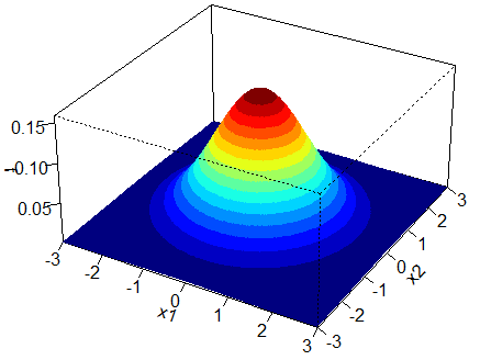
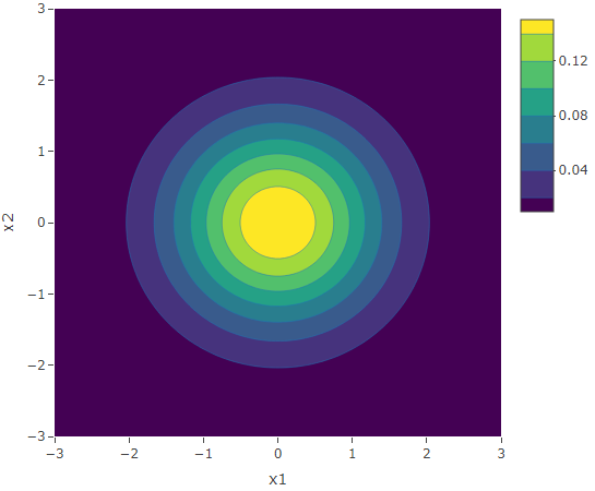
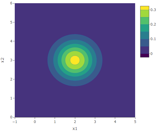
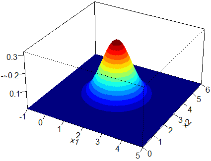
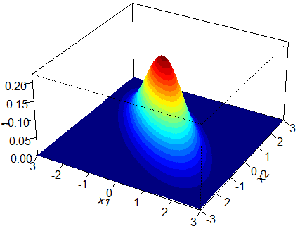
We substitute $\mu_1,\mu_2=0$ , $\sigma_{11},\sigma_{22}=1$ and $\sigma_{12}=0$ in Equation (1) and obtain the following 3D plot and contour plot. The shape of the bivariate normal distribution is again similar to a that of a bell. The multivariate normal distribution reaches its peak at $(\mu_1,\mu_2)$ . Thus in this example, the maximum is reached at $(0,0)$ . Here, since $X_1$ and $X_2$ are uncorrelated, the contours formed are perfect circles.

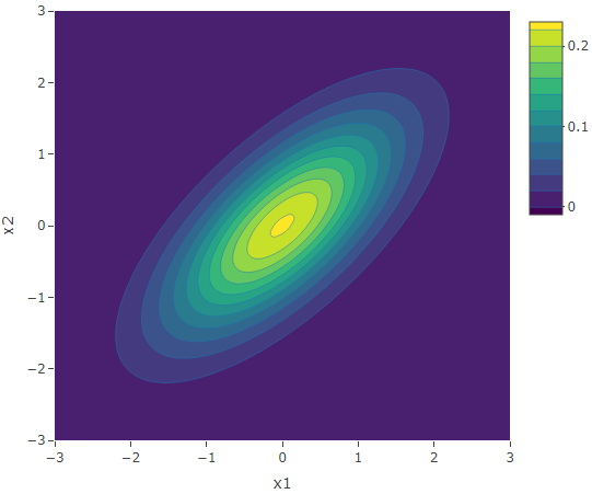
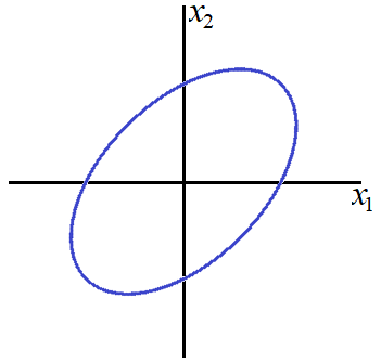
Case 2: $X_1,X_2\sim\mathcal{N}(0,1)$ with correlation 0.7.

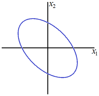
Since $\rho=0.7$ and $\sigma_{12}=\rho\sqrt{\sigma_{11}\sigma_{22}}$ , then $\sigma_{12}=0.7$ . By inputting the values of the means, variances and covariances in Equation (1), we obtain the following plots. Again we obtain a bell-shaped bivariate distribution. Since the correlation between $X_1$ and $X_2$ is positive, we obtain elliptical contours. It is like taking the circular contours of the uncorrelated case and elongate them along the diagonal $x_2=x_1$ .

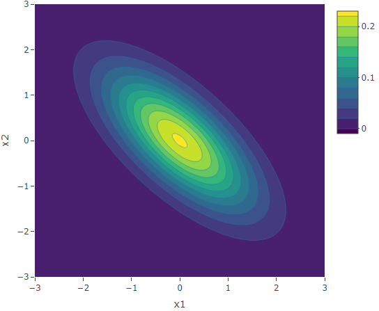
Case 3: $X_1,X_2\sim\mathcal{N}(0,1)$ with correlation -0.7.

The following are the plots for the case when the correlation is negative. Similar to the second case, we have elliptical contours. However in this case, the circular contours are elongated along the second diagonal, that is, the line $x_2=-x_1$ .

The two marginal distributions of the Bivariate Normal Distribution

Let $X_1$ and $X_2$ have a joint (combined) distribution which is the bivariate normal distribution. In general, the variable $X_1$ and $X_2$ have a correlation $\rho$ (where $\rho=\frac{\sigma_{12}}{\sqrt{\sigma_{11}\sigma_{22}}}$ ) between them, unless $\sigma_{12}=0$ . For example, when $\rho$ is positive correlation, if we known that $X_1$ resulted in a large value, then probably $X_2$ will also be large. Thus the knowledge of the value of one variable would affect the distribution of the other variable.

On the other hand, suppose we would like to know the distribution of one of the variables even though no information is given about the other variable. This would be the marginal distribution. Since we have two variables ( $X_1$ and $X_2$ ), we have two marginal distributions. The distribution of $X_1$ without any knowledge of $X_2$ is called the marginal distribution of $X_1$ . The distribution of $X_2$ without any knowledge of $X_1$ is called the marginal distribution of $X_2$ . The marginal distribution of a variable is obtained by summing the joint distribution over the other variable, as follows.

Let $g(x_1)$ be the marginal distribution of $X_1$ . Then:

$\begin{equation*} \begin{split} g(x_1)&=\int_{-\infty}^{\infty} f(x_1,x_2)dx_2\\ &=\int_{-\infty}^{\infty} \frac{1}{2\pi\sqrt{\sigma_{11}\sigma_{22}-\sigma_{12}^2}}e^{-\frac{\sigma_{22}(x_1-\mu_1)^2+\sigma_{11}(x_2-\mu_2)^2-2\sigma_{12}(x_1-\mu_1)(x_2-\mu_2)}{2(\sigma_{11}\sigma_{22}-\sigma_{12}^2)}} dx_2\\ &=\frac{1}{\sqrt{2\pi\sigma_{11}}}e^{-\frac{(x_1-\mu_1)^2}{2\sigma_{11}}}. \end{split} \end{equation*}$

The derivation involves a good number of steps with simple algebra and the use of the formula $\int_{-\infty}^{\infty}e^{-\frac{(x-\mu)^2}{2\sigma^2}}dx=\sqrt{2\pi\sigma^2}$ for any $\mu$ and $\sigma>0$ , when integrating out $x_2$ . Similarly, the marginal distribution of $X_2$ is given by:

$\begin{equation*} \begin{split} h(x_1)&=\int_{-\infty}^{\infty} f(x_1,x_2)dx_1\\ &=\int_{-\infty}^{\infty} \frac{1}{2\pi\sqrt{\sigma_{11}\sigma_{22}-\sigma_{12}^2}}e^{-\frac{\sigma_{22}(x_1-\mu_1)^2+\sigma_{11}(x_2-\mu_2)^2-2\sigma_{12}(x_1-\mu_1)(x_2-\mu_2)}{2(\sigma_{11}\sigma_{22}-\sigma_{12}^2)}} dx_1\\ &=\frac{1}{\sqrt{2\pi\sigma_{22}}}e^{-\frac{(x_2-\mu_2)^2}{2\sigma_{22}}}. \end{split} \end{equation*}$

The correlation $\rho$ (or the covariance $\sigma_{22}$ ) is not involved in the marginal distributions. The two marginal distributions can be thought of being the two building blocks of the bivariate normal distribution. In the example above where we constructed three cases of bivariate normal distribution from two standard normal random variables, the three distributions all have the same marginal distributions, but their shape is different due to the different choice of $\rho$ .

More understanding of the shape of the Bivariate Normal Distribution

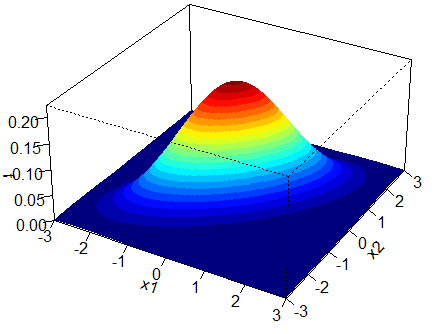
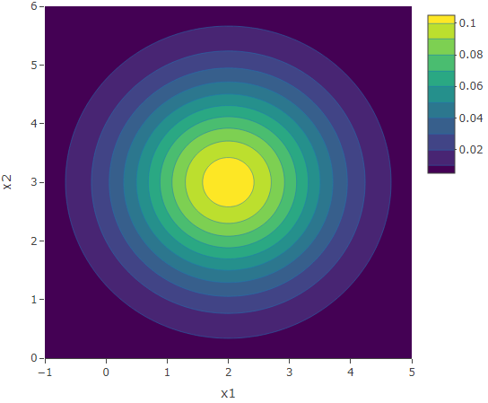
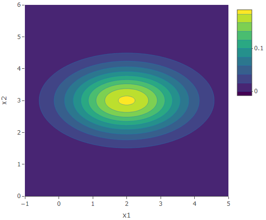
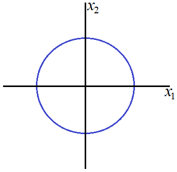
We have already seen that if the two marginal distributions are $\mathcal{N}(0,1)$ and $\rho=0$ , the contours are circular. We can generalise this. If the two marginal distributions have equal variance and $\rho=0$ , then the contours are circular. The following is the contour and 3D plot of the bivariate normal distribution with marginals $\mathcal{N}(2,1)$ and $\mathcal{N}(3,1)$ and $\rho=0$ .

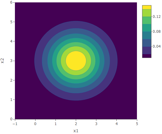
If we compare these plots with the ones of the uncorrelated standard normal marginals (the first contour and 3D plot), we see that the shape does not change. The only change is just a shift in the axis. The peak changes from $(0,0)$ to $(2,3)$ but the structural shape remains the same. This is a generalisation of the univariate case in which we have also seen that $\mu$ does not change the structure. Now consider the bivariate normal distribution with marginals $\mathcal{N}(2,0.5)$ and $\mathcal{N}(3,0.5)$ and $\rho=0$ . Also consider the bivariate normal distribution with marginals $\mathcal{N}(2,1.5)$ and $\mathcal{N}(3,1.5)$ and $\rho=0$ . These are the contour plots.

These two bivariate distributions both have no correlation present and their marginals have equal variances. Hence their contours remain circular. When the variances are small, the contours are more concentrated and vice-versa. Now let’s have a look at their respective 3D plots.

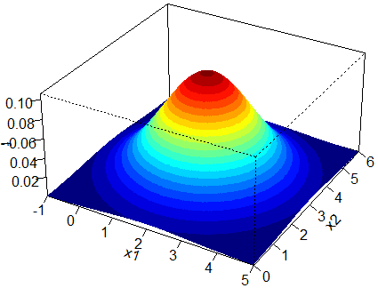
The left plot has narrower tails due to the smaller variances value and the right plot has wider tails due to the larger variances values.

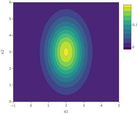
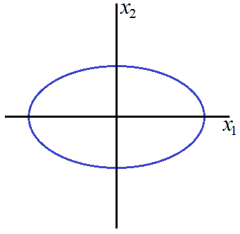
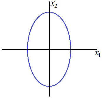
Now suppose that $\rho$ is still 0 but the variances are unequal. If $\sigma_{11}>\sigma_{22}$ , then we get elliptical contours which are circles elongated along the $x_1$ -axis. On the other hand, if $\sigma_{22}>\sigma_{11}$ , then we get elliptical contours which are circles elongated along the $x_2$ -axis. The contour plot on the left is that of the bivariate normal distribution with marginals $\mathcal{N}(2,1.5)$ and $\mathcal{N}(3,0.5)$ and $\rho=0$ . The contour plot on the right is that of the bivariate normal distribution with marginals $\mathcal{N}(2,0.5)$ and $\mathcal{N}(3,1.5)$ and $\rho=0$ .

In the general case, when $\rho$ is non-zero, there will be elongation along the either one of the two diagonals.

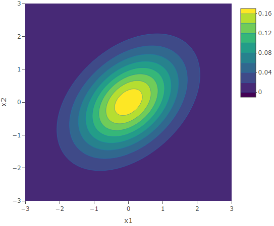
We have already seen that the positive correlation results in elongation along the main diagonal ( $x_2=x_1$ ) and a negative correlation results in elongation along the second diagonal ( $x_2=x_1$ ). Now let us have a look at the effect of the magnitude of correlation. The plot on the left is that of the bivariate normal distribution with marginals $\mathcal{N}(0,1)$ and covariance 0.4 (thus correlation 0.4). The plot on the right is that of the bivariate normal distribution with marginals $\mathcal{N}(0,1)$ and covariance 0.9 (thus correlation 0.9).

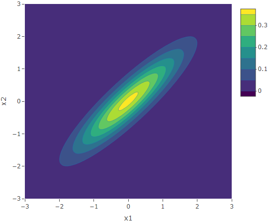
We see that a higher correlation magnitude results in elliptical contours having a shorter length (along the second diagonal $x_2=-x_1$ ), and vice-versa.

The theory behind the shape of the contours

Recall that a contour is the set of the points that have an equal function value. Hence the tuples $(x_1,x_2)$ that satisfy the equation:

$\begin{equation*} f(x_1,x_2)=k, \end{equation*}$

where $k$ is a positive number (less than the maximum value of $f$ which is $\frac{1}{2\pi\sqrt{\sigma_{11}\sigma_{22}-\sigma_{12}^2}}$ ), form a contour. We are interested in the shape of the contours of the bivariate normal distribution and how it is affected by its parameters, namely, $\mu_1$ , $\sigma_{11}$ , $\mu_2$ , $\sigma_{22}$ and $\sigma_{12}$ . We have:

$\begin{equation*} \begin{split} f(x_1,x_2)&=k\\ \frac{1}{2\pi\sqrt{\sigma_{11}\sigma_{22}-\sigma_{12}^2}}e^{-\frac{\sigma_{22}(x_1-\mu_1)^2+\sigma_{11}(x_2-\mu_2)^2-2\sigma_{12}(x_1-\mu_1)(x_2-\mu_2)}{2(\sigma_{11}\sigma_{22}-\sigma_{12}^2)}}&=k\\ e^{-\frac{\sigma_{22}(x_1-\mu_1)^2+\sigma_{11}(x_2-\mu_2)^2-2\sigma_{12}(x_1-\mu_1)(x_2-\mu_2)}{2(\sigma_{11}\sigma_{22}-\sigma_{12}^2)}}&=2k\pi\sqrt{\sigma_{11}\sigma_{22}-\sigma_{12}^2}\\ -\frac{\sigma_{22}(x_1-\mu_1)^2+\sigma_{11}(x_2-\mu_2)^2-2\sigma_{12}(x_1-\mu_1)(x_2-\mu_2)}{2(\sigma_{11}\sigma_{22}-\sigma_{12}^2)}&=\ln{2k\pi\sqrt{\sigma_{11}\sigma_{22}-\sigma_{12}^2}}\\ \sigma_{22}(x_1-\mu_1)^2+\sigma_{11}(x_2-\mu_2)^2-2\sigma_{12}(x_1-\mu_1)(x_2-\mu_2)&=-2(\sigma_{11}\sigma_{22}-\sigma_{12}^2)\ln{2k\pi\sqrt{\sigma_{11}\sigma_{22}-\sigma_{12}^2}}\\ \sigma_{22}(x_1-\mu_1)^2+\sigma_{11}(x_2-\mu_2)^2-2\sigma_{12}(x_1-\mu_1)(x_2-\mu_2)&=c, \end{split} \end{equation*}$

where $c$ ( $c>0$ ) is the constant $-2(\sigma_{11}\sigma_{22}-\sigma_{12}^2)\ln{2k\pi\sqrt{\sigma_{11}\sigma_{22}-\sigma_{12}^2}}$ .

Let us consider two cases. One where correlation is not present and the other where correlation is present

Case 1: No correlation

In this case $\sigma_{12}=0$ and the contour equation reduces to:

$\begin{equation*} \begin{split} \sigma_{22}(x_1-\mu_1)^2+\sigma_{11}(x_2-\mu_2)^2&=c\\ \frac{(x_1-\mu_1)^2}{\frac{1}{\sigma_{22}}}+\frac{(x_2-\mu_2)^2}{\frac{1}{\sigma_{11}}}&=c\\ \frac{(x_1-\mu_1)^2}{\frac{c}{\sigma_{22}}}+\frac{(x_2-\mu_2)^2}{\frac{c}{\sigma_{11}}}&=1 \end{split} \end{equation*}$

Case 1 is again broken down into 3 sub-cases: $\sigma_{11}=\sigma_{22}$ , $\sigma_{11}>\sigma_{22}$ and $\sigma_{11}<\sigma_{22}$ .

Case 1a: $\sigma_{12}=0$ and $\sigma_{11}=\sigma_{22}$

The contour equation for this sub-case becomes:

$\begin{equation*} \begin{split} \frac{(x_1-\mu_1)^2}{\frac{1}{\sigma_{11}}}+\frac{(x_2-\mu_2)^2}{\frac{1}{\sigma_{11}}}&=c\\ (x_1-\mu_1)^2+(x_2-\mu_2)^2&=\frac{c}{\sigma_{11}}. \end{split} \end{equation*}$

This is equation of a circle with centre $(\mu_1,\mu_2)$ and radius $\sqrt{\frac{c}{\sigma_{11}}}$ .

Case 1b: $\sigma_{12}=0$ and $\sigma_{11}>\sigma_{22}$

We have an ellipse with centre $(\mu_1,\mu_2)$ , width $\frac{2\sqrt{c}}{\sqrt{\sigma_{22}}}$ and length $\frac{2\sqrt{c}}{\sqrt{\sigma_{11}}}$ . Here we have $\frac{1}{\sigma_{11}}<\frac{1}{\sigma_{22}}$ and thus the width of the ellipse is greater than the height of the ellipse.

Case 1c: $\sigma_{12}=0$ and $\sigma_{11}<\sigma_{22}$

Again, we have an ellipse with centre $(\mu_1,\mu_2)$ , width $\frac{2\sqrt{c}}{\sqrt{\sigma_{22}}}$ and length $\frac{2\sqrt{c}}{\sqrt{\sigma_{11}}}$ , but since $\frac{1}{\sigma_{11}}>\frac{1}{\sigma_{22}}$ , the width of the ellipse is smaller than the height of the ellipse.

Case 2: Correlation is non-zero

Case 2 is broken down into 2 subcases: one in which the variances are equal and one in which the variances are not equal.

Case 2a: $\sigma{12}\neq 0$ and $\sigma_{11}=\sigma_{12}$

The contour equation becomes:

$\begin{equation*} \sigma_{11}(x_1-\mu_1)^2+\sigma_{11}(x_2-\mu_2)^2-2\sigma_{12}(x_1-\mu_1)(x_2-\mu_2)&=c\\ (x_1-\mu_1)^2+(x_2-\mu_2)^2-2\rho(x_1-\mu_1)(x_2-\mu_2)&=\frac{c}{\sigma_11}. \end{equation*}$

If $\rho$ (or $\sigma_{12}$ ) is positive, the equation is that of a rotated ellipse with angle $45^{\circ}$ . Hence the shape is an elongated circle along the main diagonal $x_2=x_1$ .

If $\rho$ (or $\sigma_{12}$ ) is negative, the equation is that of a rotated ellipse with angle $-45^{\circ}$ . Hence the shape is an elongated circle along the second diagonal $x_2=-x_1$ .

Case 2b $\sigma{12}\neq 0$ and $\sigma_{11}\neq\sigma_{12}$

This would be the general case and results in a rotate ellipse.

The two conditional distributions of the Bivariate Normal Distribution

We have seen that the marginal distribution is the distribution of a variable without knowing any information about the other variable. On the other hand, the conditional distribution is the distribution of a variable given the knowledge of the value of the other variable. The conditional distribution of $X_1$ given that $X_2=x_2$ is given by:

$\begin{equation*} \begin{split} g(x_1|x_2)&= \frac{f(x_1,x_2)}{g(x_2)}\\ &=\frac{\frac{1}{2\pi\sqrt{\sigma_{11}\sigma_{22}-\sigma_{12}^2}}e^{-\frac{\sigma_{22}(x_1-\mu_1)^2+\sigma_{11}(x_2-\mu_2)^2-2\sigma_{12}(x_1-\mu_1)(x_2-\mu_2)}{2(\sigma_{11}\sigma_{22}-\sigma_{12}^2)}}}{\frac{1}{\sqrt{2\pi\sigma_{22}}}e^{-\frac{(x_2-\mu_2)^2}{2\sigma_{22}}}}\\ &=\frac{1}{\sqrt{2\pi}\sqrt{\sigma_{11}-\frac{\sigma_{12}^2}{\sigma_{22}}}}e^{-\frac{(x_1-(\mu_1+\frac{\sigma_{12}}{\sigma_{22}}(x_2-\mu_2)))^2}{2(\sigma_{11}-\frac{\sigma_{12}^2}{\sigma_{22}})}}. \end{split} \end{equation*}$

Hence,

$\begin{equation*} X_1|X_2\sim\mathcal{N}(\mu_1+\frac{\sigma_{12}}{\sigma_{22}}(x_2-\mu_2),\sigma_{11}-\frac{\sigma_{12}^2}{\sigma_{22}}}). \end{equation*}$

Similarly,

$\begin{equation*} X_2|X_1\sim\mathcal{N}(\mu_2+\frac{\sigma_{12}}{\sigma_{11}}(x_1-\mu_1),\sigma_{22}-\frac{\sigma_{12}^2}{\sigma_{11}}}). \end{equation*}$

Consider the case when there is no correlation present. Therefore let us substitute $\sigma_{12}=0$ in the above two equations. We obtain:

$\begin{equation*} X_1|X_2\sim\mathcal{N}(\mu_1,\sigma_{11})\mbox{ and }X_2|X_1\sim\mathcal{N}(\mu_2,\sigma_{22}). \end{equation*}$

Thus the conditional distributions are simply the marginal distribution in the case when $\rho=0$ . When there is no correlation, the distribution of one of the variables is the same with or without the knowledge of the value of the other variable. Note that in $X_1|X_2$ , the value of $X_2$ affects the mean but not the variance. The variance of $X_1|X_2$ is constant no matter the choice of value of $X_2$ . Similar analysis could be made for the random variable $X_2|X_1$ .

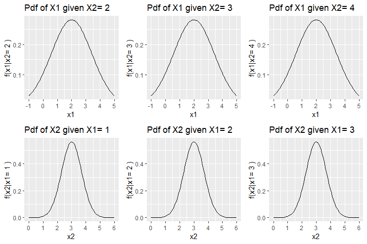
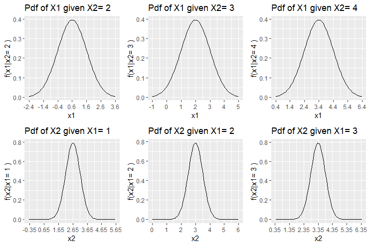
Let us consider some examples of bivariate normal distributions and have a look at 6 conditional distributions presented in a grid. The first 3 are plots of $X_1|X_2$ when $X_2=\mu_2-1,\mu_2$ and $\mu_2+1$ . The last 3 are plots of $X_2|X_1$ when $X_1=\mu_1-1,\mu_1$ and $\mu_1+1$ .

Example 1: $X_1\sim\mathcal{N}(2,2)$ , $X_1\sim\mathcal{N}(3,0.5)$ and $\rho=\sigma_{12}=0$

The following is the contour plot of this bivariate distribution. The 6 lines correspond to 6 cross-sections of the distribution. A cross-section along a horizonal or vertical line and scaling the area to be equal to 1, results in a conditional distribution. The 3 pink horizontal ones correspond to the probability distributions of $X_1|X_2=2$ , $X_1|X_2=3$ and $X_1|X_2=4$ . The 3 red vertical ones corresponds to the probability distributions of $X_2|X_1=1$ , $X_2|X_1=2$ and $X_2|X_1=3$ .

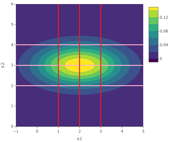
As we already mentioned, since the correlation is zero, the conditional distribitions of $X_1|X_2$ are all the same and equal to the marginal distribution of $X_1$ . In fact the first 3 are all equal to the first marginal distribution $\mathcal{N}(2,2)$ and the last 3 are all equal to the second marginal distribution $\mathcal{N}(3,0.5)$ .

Example 2: $X_1\sim\mathcal{N}(2,2)$ , $X_1\sim\mathcal{N}(3,0.5)$ and $\rho=0.7$

This is an example in which the correlation is positive. In this case $\sigma_{12}=\rho\sqrt{\sigma_{11}}\sqrt{\sigma_{22}}=\rho\sqrt{2}\sqrt{0.5}=\rho=0.7$ . The following is the contour plot.

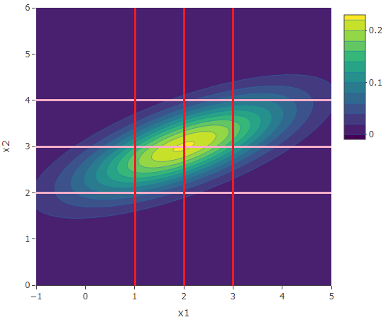
Consider the plots of the conditional distributions. In the first plot, the value of $X_2$ is 2 which is less than $\mu_2=3$ . Hence since the correlation is positive we expect that $X_1$ (given that $X_2=2$ ) takes a value less than the mean $\mu_1=2$ . In fact the mean of $X_1|X_2=0.6$ which is less than $\mu_1$ . The knowlegde that $X_2$ took a small value, will give us a hint that $X_1$ will also take a small value, due to a positive correlation.

Example 3: $X_1\sim\mathcal{N}(2,2)$ , $X_1\sim\mathcal{N}(3,0.5)$ and $\rho=-0.7$

Here we have a negative correlation. The following is the contour plot of this bivariate normal distribution.

Consider the plots of the conditional distributions. In particular, in the first plot, the value of $X_2$ is 2 which is less than $\mu_2=3$ . Since the correlation is negative we expect that $X_1$ (given that $X_2=2$ ) takes a value greater than the mean $\mu_1=2$ . In fact the mean of $X_1|X_2=3.4$ which is more than $\mu_1$ . The knowlegde that $X_2$ took a small value, will give us a hint that $X_1$ will take a larger value (with respect to the mean $\mu_1$ ), due to the negative correlation.

We have noted that there is no change in the variance of $X_1|X_2$ (or $X_2|X_1$ ) with the change of the value of $X_2$ (or $X_1$ respectively). Hence in the grid of plots, all the plots in the same row has the same shape (because it is the variance that changes the shape of the graph of the normal distribution). There are other ways how to combine two marginal distribution to form a bivariate distribution. One of these ways is by using copulas, which is a generalised way how to combine two distributions (in particular normal distributions) that allow for a variance structure which is not constant over the value of the conditioned variable.

Conclusion

In this article, we showed different 3D and contour plots of bivariate normal distributions. We have seen the conditions that make a bivariate normal distribution have particular contour structure, like circular, elliptical and rotated elliptical structure. We analysed the structure of the conditional distribution of a bivariate normal distribution with no correlation present, with positive correlation and negative correlation. In particular, we have seen that the variance of the conditional distribution remains constant over the different values of the conditioned variable. This leads to the study of copulas, which allow a variable structure for the conditional distribution, when combining two distributions.

Appendix: R Code

Here we will present the codes used in the article, together with some explanations. The following is the code for a 3D plot of the bivariate normal distribution. It requires the package GA (Genetic Algorithms). The input parameters consist of $\mu_1$ , $\mu_2$ , $\sigma_{11}$ , $\sigma_{22}$ and $\sigma_{12}$ . The range of the $x_1$ -axis is set to 3 units around its mean $\mu_1$ and the same for the $x_2$ -axis. Note that in the function “persp3D”, the variables “theta” and “phi” specify the angle at which we are looking at the plot.

library(GA)

#input
mu1<-2 #mean of X_1
mu2<-10 #mean of X_2
sigma11<-1 #variance of X_1
sigma22<-0.5 #variance of X_2
sigma12<-0 #covariance of X_1 and X_2 

#plot
x1 <- seq(mu1-3, mu1+3, length= 500)
x2 <- seq(mu2-3, mu2+3, length= 500)
z <- function(x1,x2){ z <- exp(-(sigma22*(x1-mu1)^2+sigma11*(x2-mu2)^2-2*sigma12*(x1-mu1)*(x2-mu2))/(2*(sigma11*sigma22-sigma12^2)))/(2*pi*sqrt(sigma11*sigma22-sigma12^2)) }
f <- outer(x1,x2,z)
persp3D(x1, x2, f, theta = 30, phi = 30, expand = 0.5)

The following is the R code for the contour plot of the bivariate normal distribution. This makes use of the package plotly.

library(plotly)

#input
mu1<-2 #mean of X_1
mu2<-3 #mean of X_2
sigma11<-0.5 #variance of X_1
sigma22<-1.5 #variance of X_2
sigma12<-0 #covariance of X_1 and X_2 

#plot
x1 <- seq(mu1-3, mu1+3, length= 100)
x2 <- seq(mu2-3, mu2+3, length= 100)
z <- function(x1,x2){ z <- exp(-(sigma22*(x1-mu1)^2+sigma11*(x2-mu2)^2-2*sigma12*(x1-mu1)*(x2-mu2))/(2*(sigma11*sigma22-sigma12^2)))/(2*pi*sqrt(sigma11*sigma22-sigma12^2)) }
f <- t(outer(x1,x2,z))

plot_ly(x=x1,y=x2,z=f,type = "contour")%>%layout(xaxis=list(title="x1"),yaxis=list(title="x2"))

The following is the R code for the plot of the conditional distribution $X_1|X_2$ . This makes use of the package ggplot2. Note that the input requires also a fixed value of $X_2$ .

library(ggplot2)

#input
mu1<-2 #mean of X_1
mu2<-3 #mean of X_2
sigma11<-2 #variance of X_1
sigma22<-0.5 #variance of X_2
sigma12<-0.4 #covariance of X_1 and X_2 
x2<-4 #the fixed value of X_2

#plot
x1<-seq(round(mu1+sigma11*(x2-mu2)/sigma22,1)-3,round(mu1+sigma11*(x2-mu2)/sigma22,1)+3,length=100)
Curve<-dnorm(x1, mean =mu1+sigma11*(x2-mu2)/sigma22, sd = sigma11-(sigma12^2)/sigma11)
NormalDistData<-data.frame(x1,Curve)
ggplot()+geom_line(data=NormalDistData,aes(x=x1,y=Curve))+ scale_x_continuous(breaks = seq(mu1+sigma11*(x2-mu2)/sigma22-3,mu1+sigma11*(x2-mu2)/sigma22+3,by=1))+ylab(paste("f(x1|x2=",as.character(x2),")"))+ggtitle(paste("Pdf of X1 given X2=",as.character(x2)))